library(rvest)
library(RSelenium)
library(dplyr)Recently, I came across an web article titled 65 Funny Town Names Across the U.S.1. Ever since I started living in the states, I was awed by the simultaneous banality and eccentricity of the country’s town names. As I was scrolling through the ad explosion of the article, I kept wondering what one has to do make such a list and also whether the list covers all the funny town names after all. So I decided to do this fun endeavor. Here are a few street views showcasing some of the interesting names I found.
Fire Station in Moody, Alabama
THE TOWN OF MAN
A water tank located in Magazine, Arkansas
The endeavor would be incomplete if I don’t list the names from the article first. But the invasive advertisement made it hard for me to scroll any farther down and I decided to scrape from the web article using RSelenium2.
link <- "https://www.farandwide.com/s/wacky-town-names-47d4c1c59a624a70"I run the following command from the terminal to start the Docker container which will act like a server docker run -d -p 4445:4444 selenium/standalone-firefox. Then I use RSelenium to launch a headless browser from the server which will read the article for me. The browser loads the webpage and keeps pressing End key to scroll down and get a glimpse of everything. Finally, it collects the names from the element of interest.
system("docker run -d -p 4445:4444 selenium/standalone-firefox")remDr <- remoteDriver(
remoteServerAddr = "localhost",
port = 4445L,
browserName = "firefox"
)remDr$open()remDr$navigate(link)This is where the browser keeps scrolling down.
webElem <- remDr$findElement("xpath", "/html/body")

# Scroll down 10 times
for(i in 1:10){
  webElem$sendKeysToElement(list(key = "end"))
  # please make sure to sleep a couple of seconds because it takes time to load contents
  Sys.sleep(5)
}
page_source <- remDr$getPageSource()I used inspect on my real browser to discover the fact that list-item-title is the element/node I am looking for. That is primarily because I am a noob. I am sure any decent-skilled web scraper would have found a smart way to do it from the headless browser.
all_funny_names <- read_html(page_source[[1]]) %>% html_nodes(".list-item-title") %>% html_text()Looks like we got 2 titles. There may have been similar elements in the web page that we don’t want. Since, the article says 65 town names let’s peek at the values from 61-70 and decide where to cut-off.
(all_funny_names$x %>% head(70) %>% tail(10)) [1] "Why, Arizona" "Whynot, North Carolina" "Yum Yum, Tennessee"
[4] "Zigzag, Oregon" "Zzyzx, California" "Branson, Missouri"
[7] "Where to Stay" "Baraboo, Wisconsin" "Where to Stay"
[10] "Brainerd, Minnesota" Looks like it ends with Zzyzx, California or at index 65. Others are promotional towns featured in the article. Let’s filter everything after the 65th one.
all_funny_names <- all_funny_names[1:65,]Here’s the final list.
all_funny_names$x [1] "Accident, Maryland" "Aladdin, Wyoming"
[3] "Bacon Level, Alabama" "Bat Cave, North Carolina"
[5] "Bigfoot, Texas" "Bitter End, Tennessee"
[7] "Booger Hole, West Virginia" "Boring, Oregon"
[9] "Breeding, Kentucky" "Bugtussle, Kentucky"
[11] "Burnout, Alabama" "Carefree, Arizona"
[13] "Center of the World, Ohio" "Chicken, Alaska"
[15] "Coke County, Texas" "Cookietown, Oklahoma"
[17] "Correct, Indiana" "Cut and Shoot, Texas"
[19] "Ding Dong, Texas" "DISH, Texas"
[21] "Early, Iowa" "Earth, Texas"
[23] "Fifty-Six, Arkansas" "Frankenstein, Missouri"
[25] "French Lick, Indiana" "Funk, Nebraska"
[27] "Good Grief, Idaho" "Greasy Corner, Arkansas"
[29] "Half Hell, North Carolina" "Hell, Michigan"
[31] "Hot Coffee, Mississippi" "Hurt, Virginia"
[33] "Hygiene, Colorado" "Intercourse, Pennsylvania"
[35] "Ketchuptown, South Carolina" "Knockemstiff, Ohio"
[37] "Monkey’s Eyebrow, Kentucky" "Neutral, Kansas"
[39] "No Name, Colorado" "Normal, Illinois"
[41] "Nothing, Arizona" "Peculiar, Missouri"
[43] "Pee Pee, Ohio" "Pfafftown, North Carolina"
[45] "Plastic, Colorado" "Poverty, Kentucky"
[47] "Random Lake, Wisconsin" "Romance, Arkansas"
[49] "Rough and Ready, California" "Santa Claus, Indiana"
[51] "Satan's Kingdom, Massachusetts" "Slaughterville, Oklahoma"
[53] "Scratch Ankle, Alabama" "Success, Missouri"
[55] "Tombstone, Arizona" "Top-of-the-World, Arizona"
[57] "Truth or Consequences, New Mexico" "Turkey Scratch, Arkansas"
[59] "Two Egg, Florida" "Wealthy, Texas"
[61] "Why, Arizona" "Whynot, North Carolina"
[63] "Yum Yum, Tennessee" "Zigzag, Oregon"
[65] "Zzyzx, California" This web article is certainly not the first one to march this direction. A quick Google search gave me a book titled The Cafeteria Lady Eats Her Way Across America: And Lives to Tell About It!3 which has a chapter “A Town By Any Other Name” dedicated to stringing these names together into a narrative. Luckily, these pages are available for preview in the Google books website so if anybody wants they can check it out. There’s also a line in one of the Wrens’ song “Why into Whynot” but I have no proof they meant the towns Why, Arizona and Whynot, North Carolina.
Inspired by these, I wanted to make a comprehensive list of all the names. So I went looking for the largest list of US town names available in the internet. There were quite a few and one from the Github4 had 60k+ records. Of course, I am not going to comb through this list so I started thinking of better approaches.
The first idea that I had was to use a dictionary. Most of the words in the web article and the book were actually dictionary words except for a few goofy ones. So I decided to use the hunspell5 library to filter out town names that are not dictionary words.
all_town_df <- read.csv('us_cities_states_counties.csv', sep="|")library(hunspell)selected_indices <- all_town_df$City.alias %>% hunspell_check(dict=dictionary("en_US"))
all_town_df_filtered <- all_town_df %>% filter(selected_indices)That didn’t help much. We still have 63210 entries left. But most of them should be duplicates and a lot of them could have a really high frequency (think Springfield). We are not interested in the high frequency ones, good things come in small portion. Let’s use table() then hist() to see the frequency distribution.
frequency_table <- table(all_town_df_filtered$City.alias)
hist(frequency_table)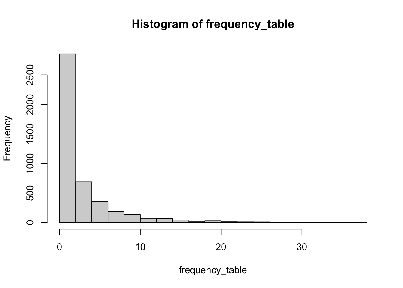
We still have a lot of town names that are not frequent but still a dictionary word. Let’s say any town name that appears more than 4 times is more or less accepted by the people as a common town name and filter those out.
less_common_town_names <- names(frequency_table[frequency_table <= 4])
all_town_df_filtered <- all_town_df_filtered %>% filter(City.alias %in% less_common_town_names)
There’s still 3547 town names left for us to comb through. Now I want to see some of the names to come up with an idea on how to proceed.
less_common_town_names %>% head(50) [1] "88" "Aaron" "Abbot" "Abel" "Abernathy"
[6] "Abilene" "Abraham" "Abram" "Abrams" "Academia"
[11] "Academy" "Accident" "Accord" "Ace" "Achilles"
[16] "Acorn" "Acosta" "Action" "Adamant" "Adelaide"
[21] "Aden" "Adirondack" "Adkins" "Admire" "Adolph"
[26] "Advance" "Advent" "Aeneas" "Africa" "Agana"
[31] "Agar" "Agate" "Agency" "Agenda" "Ages"
[36] "Agnes" "Agnew" "Agra" "Agricola" "Aguilar"
[41] "Aguirre" "Aiken" "Ajax" "Akin" "Alabama"
[46] "Alabaster" "Aladdin" "Alamogordo" "Alaska" "Albee" As much as it is interesting to hear about Alabama, New York, I am looking for something that gives a stronger kick upon hearing it. There are enough Paris, Texas references in the world for it to have become trivial by now. There are also people names such as Abraham, Agnes, Adolph that are in the hunspell dictionary that are better off being filtered. In fact, therein lies the problem. hunspell dictionary is too much inclusive for our task. We need a dictionary that is less interested in the proper nouns.
After looking around for a while, I found the freeDictionaryAPI6 which can be queried using the url https://api.dictionaryapi.dev/api/v2/entries/en/{word}. So I initially tried to use url_exists() function of RCurl library but that ended up in Error 429 (too many requests). I could have used Sys.sleep() but I decided to poke around the freeDictionaryAPI looking for ways to query with multiple words. I found something even better. There is a word list directly available in their Github page.
dictionary_file <- file('freeDictionaryAPI.txt')
freeDictionaryAPI_words <- readLines(dictionary_file)
close(dictionary_file)
Now let’s run the function over less_common_town_names and filter based on the result. I am using purrr::map_lgl() to avoid writing a loop in this case.
words_with_definition <- tolower(less_common_town_names) %in% freeDictionaryAPI_wordstown_names <- less_common_town_names %>% subset(words_with_definition)set.seed(42)
sample(town_names, 50) [1] "Maple" "Lemons" "Moe" "Dyke" "Wrens"
[6] "Mack" "Nursery" "Windfall" "Cc" "Root"
[11] "Bighorn" "Tiffany" "Headland" "Donna" "Nineteen"
[16] "Hoard" "Irons" "Visa" "Druid" "Quay"
[21] "Gumbo" "Brothers" "Odds" "Corn" "Northwest"
[26] "Zap" "Cadillac" "Nook" "Gravity" "Ina"
[31] "Outing" "Quarry" "Fishers" "Hon" "Duke"
[36] "Bruin" "Battleground" "Panorama" "Junction" "Chaparral"
[41] "Jester" "Thorn" "Electron" "Crocus" "Altitude"
[46] "Wisdom" "Bandy" "Zinc" "Op" "Seminary" We still have 2116 names left. I printed 50 random samples above to see if this is what we were looking for from the first place. The results don’t look too bad, you definitely won’t expect most of them to be a town name. Any attempt at shortening the current list has a high probability of removing some interesting town names. That’s why I will keep it as it is for now.
Some names that really surprised me:
Tea, South Dakota
Bachelor, Missouri
Bonus, Illinois
Electron, Washington
Home, Washington
Sweet Home, Oregon
Junior, West Virginia
Leisure, Indiana
Man, West Virginia
Magazine, Arkansas
Oil, Indiana
Printer, Kentucky
Republican, Arkansas
One final thing I want to do is show the remaining towns on the OpenStreetMap7 using Leaflet8. But before I do that, I need to actually get their location. I will use ggmap9 for that.
funny_town_df <- all_town_df %>% filter(City.alias %in% town_names)funny_town_df["address"] <- paste0(funny_town_df$City.alias, ", ", funny_town_df$State.full)api_key <- "API_KEY"
library(ggmap)
register_google(api_key)funny_town_df <- funny_town_df %>% mutate_geocode(address)After the lon and lat values are retrieved, we can quickly convert it to sf.
library(sf)
library(leaflet)
library(OpenStreetMap)
library(osmdata)
funny_town_sf <- st_as_sf(funny_town_df, coords=c("lon", "lat"), crs = 4326)Google map might have looked for places with similar name elsewhere in the world when one was not found within the United States. We need to filter those out.
library(spData)
data('world')
usa_map <- world[world$name_long == "United States",]
funny_town_sf <- funny_town_sf %>% filter(lengths(st_intersects(funny_town_sf, usa_map)) > 0)(m <- leaflet() %>%
addTiles() %>%
addProviderTiles("OpenStreetMap.HOT", group = "Humanitarian") %>%
addTiles(options = providerTileOptions(noWrap = TRUE), group = "Default") %>%
# addMarkers(lng = dhaka_long, lat = dhaka_lat, popup='Dhaka') %>%
# addRectangles(bbox_val[[1]], bbox_val[[2]], bbox_val[[3]], bbox_val[[4]]) %>%
addMarkers(data=funny_town_sf, clusterOptions = markerClusterOptions()))References
1
Milling, Marla Hardee (2023) “65 funny town names across the u.s.” [online] Available from: https://www.farandwide.com/s/wacky-town-names-47d4c1c59a624a70
2
Harrison, John (2022) RSelenium: R bindings for ’selenium WebDriver’, [online] Available from: https://CRAN.R-project.org/package=RSelenium
3
Bolton, Martha (2006) The cafeteria lady eats her way across america: And lives to tell about it!, Regal Books.
4
grammakov (2014) “US cities, counties and states.” [online] Available from: https://github.com/grammakov/USA-cities-and-states
5
Ooms, Jeroen (2022) Hunspell: High-performance stemmer, tokenizer, and spell checker, [online] Available from: https://CRAN.R-project.org/package=hunspell
6
https://github.com/meetDeveloper (2019) “Free dictionary API.” [online] Available from: https://dictionaryapi.dev/
7
Fellows, Ian and JMapViewer library by Jan Peter Stotz, using the (2019) OpenStreetMap: Access to open street map raster images, [online] Available from: https://CRAN.R-project.org/package=OpenStreetMap
8
Cheng, Joe, Karambelkar, Bhaskar and Xie, Yihui (2022) Leaflet: Create interactive web maps with the JavaScript ’leaflet’ library, [online] Available from: https://CRAN.R-project.org/package=leaflet
9
Kahle, David and Wickham, Hadley (2013) “Ggmap: Spatial visualization with ggplot2.” The R Journal, 5(1), pp. 144–161. [online] Available from: https://journal.r-project.org/archive/2013-1/kahle-wickham.pdf