library(sf)
library(raster)
library(dplyr)
library(spData)
library(terra)
library(OpenStreetMap)
library(osmdata)
library(leaflet)Where to Look for Cheap Rental Flats in Dhaka
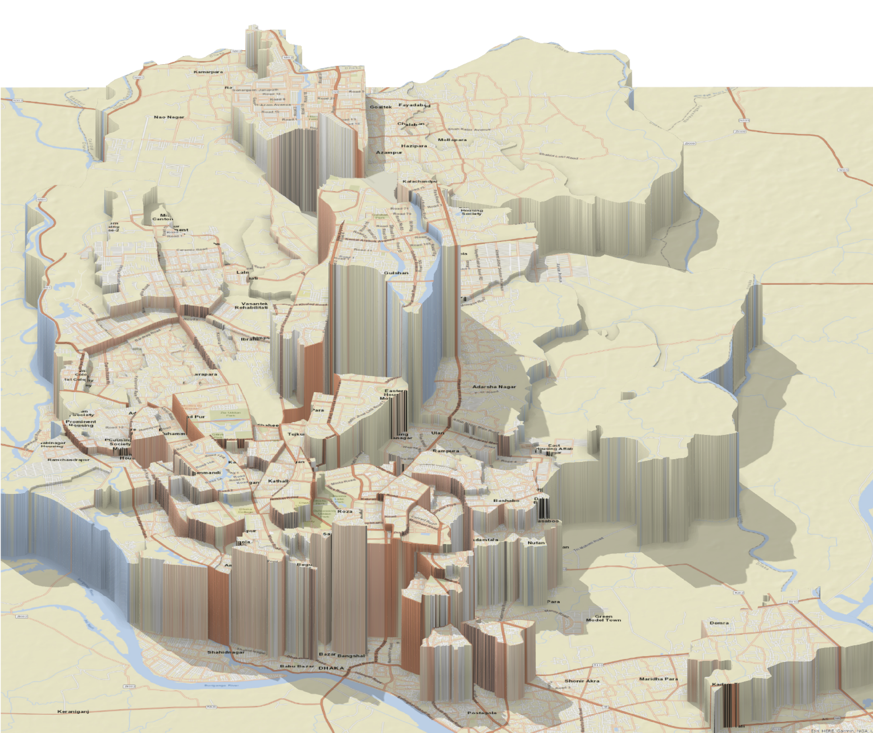
This is probably what the title of this article could have been if it was a clickbait attempt. But I think the image below serves a similar purpose. Now I will walk you through what steps I undertook to get this comparative visualization of rental apartment costs around Dhaka.
Loading the shape files of three different layers of administrative distribution. I downloaded this data from Humanitarian Data Exchange9. There are 4 different administrative area categories in Bangladesh. ADMIN1: the divisions, ADMIN2: the districts, ADMIN3: upazillas/sectors (the latter for cities), ADMIN4: unions/wards (the former for rural areas, the latter for cities). Since I am only interested in the city of Dhaka which is a part of the district Dhaka, I am only interested in the layers ADMIN3 and ADMIN4. I will also call areas from these layers as ADMIN3 area and ADMIN4 area respectively.
shape_file_3 = st_read("bgd_admbnda_adm3_bbs_20201113.shp")Reading layer `bgd_admbnda_adm3_bbs_20201113' from data source
`/Users/farganaislam/farganaislamblog/posts/dhaka-rental-listing/bgd_admbnda_adm3_bbs_20201113.shp'
using driver `ESRI Shapefile'
Simple feature collection with 544 features and 16 fields
Geometry type: MULTIPOLYGON
Dimension: XY
Bounding box: xmin: 88.00863 ymin: 20.59061 xmax: 92.68031 ymax: 26.63451
Geodetic CRS: WGS 84Only keeping the ADMIN3 areas that are situated in the Dhaka metropolitan area.
shape_file_3 = shape_file_3 %>% subset(ADM2_EN == 'Dhaka')
shape_file_3 = shape_file_3 %>% filter(Shape_Area < 1.00e-02)
ADM3_list <- as.vector(st_drop_geometry(shape_file_3['ADM3_EN']))[['ADM3_EN']]
Load ADMIN4 areas and keep only those that are inside the same area as ADM3_list
shape_file_4 = st_read("shape_file_4_small.shp")Reading layer `shape_file_4_small' from data source
`/Users/farganaislam/farganaislamblog/posts/dhaka-rental-listing/shape_file_4_small.shp'
using driver `ESRI Shapefile'
Simple feature collection with 203 features and 18 fields
Geometry type: POLYGON
Dimension: XY
Bounding box: xmin: 90.00457 ymin: 23.52215 xmax: 90.51279 ymax: 24.04435
Geodetic CRS: WGS 84shape_file_4 = shape_file_4 %>% subset(ADM2_EN == 'Dhaka')
shape_file_4p = shape_file_4 %>% subset(ADM3_EN %in% ADM3_list)Visualizing the map on leaflet
bbox_val <- st_bbox(shape_file_4p)

(m <- leaflet() %>%
  addTiles() %>%
  addProviderTiles("OpenStreetMap.HOT", group = "Humanitarian") %>%
  addTiles(options = providerTileOptions(noWrap = TRUE), group = "Default") %>%
  # addMarkers(lng = dhaka_long, lat = dhaka_lat, popup='Dhaka') %>%
  # addRectangles(bbox_val[[1]], bbox_val[[2]], bbox_val[[3]], bbox_val[[4]]) %>%
  addPolygons(data = shape_file_3, fillOpacity = 0.1, label = ~ADM3_EN, weight=1.5,
              labelOptions = labelOptions(noHide = TRUE, textOnly = TRUE, style = list("font-size"="8px", "color"="blue"))
              ))
Now let’s read the rental price data. This is from a Kaggle Dataset10. The provider scraped it from the popular website bproperty.com and released it under CC0 license.
property_data <- read.csv('property_listing_data_in_Bangladesh.csv')
summary(property_data)
title beds bath area
Length:8294 Length:8294 Length:8294 Length:8294
Class :character Class :character Class :character Class :character
Mode :character Mode :character Mode :character Mode :character
adress type purpose flooPlan
Length:8294 Length:8294 Length:8294 Length:8294
Class :character Class :character Class :character Class :character
Mode :character Mode :character Mode :character Mode :character
url lastUpdated price
Length:8294 Length:8294 Length:8294
Class :character Class :character Class :character
Mode :character Mode :character Mode :character Let’s fix the incorrect spelling of the column names.
property_data <- property_data %>% rename(address = adress) %>% rename(floorPlan = flooPlan)Initially we are only concerned with the following columns: ‘adress’, ‘area’, ‘beds’, ‘bath’, ‘price’. Let’s look at a few rows to get a good idea. Later, I will use the trick from the link https://www.cararthompson.com/posts/2022-09-09-automating-sentences-with-r/ to make the above list more dynamic
head(property_data[c('address', 'area', 'beds', 'bath', 'price')]) address area beds bath price
1 Priyanka City, Sector 12, Uttara, Dhaka 1,500 sqft 3 3 30 Thousand
2 Modhubag, Boro Maghbazar, Maghbazar, Dhaka 4 3 22 Thousand
3 Block G, Bashundhara R-A, Dhaka 1,850 sqft 3 3 35 Thousand
4 Block G, Bashundhara R-A, Dhaka 1,850 sqft 3 3 35 Thousand
5 Sector 5, Uttara, Dhaka 1,500 sqft 3 3 30 Thousand
6 Block J, Banasree, Dhaka 1,500 sqft 3 3 20 ThousandLet’s count how many of the entries are actually in Dhaka.
total_num_of_entries <- count(property_data)
(num_of_entries_in_dhaka <- grepl("Dhaka", property_data$address) %>% sum())
[1] 6092So, about 73.5 % of the entries are from Dhaka. That is good for us. Let’s filter the other entries from property_data.
property_data <- property_data %>% subset(grepl("Dhaka", property_data$address))One thing to note is that property_data does not have any spatial information. The address is a string that one is tempted to look up in a web mapping platform. In fact, I am just going to do that using Google Maps API. However, I cannot disclose my API in the open web. So as a compromise, I will write a function called pseudo_mutate_geocode that will essentially simulate the behavior of ggmap::mutate_geocode. In order to do that, I called the actual mutate_geocode function and queried Google Maps with the addresses listed in property_data. I stored the query output in a new dataframe and saved it to a csv file. The pseudo_mutate_geocode function actually reads from that csv file to simulate the same behavior. However, if you want to query Google Maps using your own API key, that option is given to you as well. All you have to do is set the api_key variable’s value to your API key.
pseudo_mutate_geocode <- function(data, location) {
  left_join(data, read.csv('cached_google_map_query.csv')[c("address", "lon", "lat")], by = location)
}

api_key <- "NO_API_KEY_PROVIDED"
if (api_key == "NO_API_KEY_PROVIDED") {
  head(property_data <- property_data %>% pseudo_mutate_geocode("address"))[c("address", "lon", "lat")]
} else {
  library(ggmap)
  register_google(api_key)
  head(property_data <- property_data %>% mutate_geocode(address))[c("address", "lon", "lat")]
}
address lon lat
1 Priyanka City, Sector 12, Uttara, Dhaka 90.37978 23.86853
2 Modhubag, Boro Maghbazar, Maghbazar, Dhaka 90.40898 23.74936
3 Block G, Bashundhara R-A, Dhaka 90.43314 23.82441
4 Block G, Bashundhara R-A, Dhaka 90.43314 23.82441
5 Sector 5, Uttara, Dhaka 90.39073 23.86467
6 Block J, Banasree, Dhaka 90.43314 23.76194head(property_data[c('address', 'lon', 'lat', 'area', 'beds', 'bath', 'price')]) address lon lat area beds
1 Priyanka City, Sector 12, Uttara, Dhaka 90.37978 23.86853 1,500 sqft 3
2 Modhubag, Boro Maghbazar, Maghbazar, Dhaka 90.40898 23.74936 4
3 Block G, Bashundhara R-A, Dhaka 90.43314 23.82441 1,850 sqft 3
4 Block G, Bashundhara R-A, Dhaka 90.43314 23.82441 1,850 sqft 3
5 Sector 5, Uttara, Dhaka 90.39073 23.86467 1,500 sqft 3
6 Block J, Banasree, Dhaka 90.43314 23.76194 1,500 sqft 3
bath price
1 3 30 Thousand
2 3 22 Thousand
3 3 35 Thousand
4 3 35 Thousand
5 3 30 Thousand
6 3 20 ThousandNow I use the lon and lat attribute as location to convert the dataframe into an sf. I also add ADM4_PCODE for each row from the shape_file_4p sf.
property_data_sf <- st_as_sf(property_data, coords=c("lon", "lat"), crs = 4326)
(number_of_rows <- count(property_data_sf)[[1]])
[1] 6092After the conversion, we have 6092 left. That means the google map query could not find location value for the other 0 rows.
Now let’s try to see which ADMIN4 area each of this location point is situated in.
property_data_sf <- st_join(property_data_sf, shape_file_4p['ADM4_PCODE'], st_intersects, left=TRUE)Let’s count the number of rows left na values we got in ADM4_PCODE when st_join could not find any admin area in which the rental property is located.
sum(is.na(property_data_sf$ADM4_PCODE))[1] 0That is really good. This means we don’t have to filter any of the rows for now.
Now let’s look at the other non-spatial attributes in property_data. Previously, we have seen all the columns are actually character strings even though some of them could benefit from being converted to numeric. There are also categorical attributes such as type and purpose. Let’s look at what are the unique possible values of these attributes and their frequencies. The columns beds and bath are not exactly categorical but they are integers and looking at their possible values could also be helpful.
lapply(property_data_sf[c('type', 'purpose', 'beds', 'bath')] %>% st_drop_geometry(), table)$type
Apartment Building Duplex
6028 19 45
$purpose
For Rent
6092
$beds
1 Bed 14 17 18 2 20 21 22 3 32 4 5 6
117 1 1 1 1957 3 2 1 3496 1 452 46 9
7
5
$bath
1 Bath 10 2 3 4 5 6 7 8
327 10 2355 2405 873 103 12 1 6 Looking at the type attribute we can see that almost all the entries are apartments. Even though we have some building and duplex rows, they are likely to skew the rent distribution. That’s why I filter entries that are not apartments.
property_data_sf <- property_data_sf %>% filter(type == 'Apartment')All the apartments are for rent so we don’t have to do anything with the purpose attribute.
‘1 Bed’ is the only value that cannot be easily converted to numeric. Same goes for ‘1 Bath’. Let’s delete the non-numeric portion in those cases using gsub. After that we convert them to numeric.
property_data_sf$beds <- gsub(pattern = '1 Bed', replacement= '1', property_data_sf$beds) %>% as.numeric()
property_data_sf$bath <- gsub(pattern = '1 Bath', replacement= '1', property_data_sf$bath) %>% as.numeric()
area and price are in character string as well and we need to convert them to numeric. We need to first identify the possible word suffixes in these attributes. Let’s use regex [0-9] to delete the numeric portion and see all the unique suffixes.
(area_suffixes <- gsub("[0-9]", "", property_data_sf$area) %>% table()).
sqft , sqft
1973 468 3587 We have 1973 rows with no suffixes and other rows contain sqft as the suffix. We also have to get rid of the ‘,’ between the digits.
property_data_sf$area <- as.numeric(property_data_sf$area %>% gsub(' sqft', '', .) %>% gsub(',', '', .))Now let’s find out the suffixes in price.
(price_suffixes <- gsub("[0-9]", "", property_data_sf$price) %>% table()).
Lakh Thousand . Lakh . Thousand
93 5424 223 288 This time we have two suffixes and depending on which of them is present, we need to multiply the numeric portion with 100000 or 1000. Let’s use a combination of grepl and gsub to achieve this.
property_data_sf$rent <- property_data_sf$price %>%
                         gsub(" Thousand", "", .) %>%
                         gsub(" Lakh", "", .) %>%
                          as.numeric() *
                         (1000*(property_data_sf$price %>% grepl(" Thousand", .))
                           +100000*(property_data_sf$price %>% grepl(" Lakh", .)))
I rename this as rent since it suits the context better.
Let’s look at the summary of the 4 numerical attributes.
summary(property_data_sf[c('beds', 'bath', 'area', 'rent')] %>% st_drop_geometry()) beds bath area rent
Min. :1.000 Min. :1.000 Min. : 600 Min. : 7000
1st Qu.:2.000 1st Qu.:2.000 1st Qu.: 1150 1st Qu.: 15000
Median :3.000 Median :3.000 Median : 1300 Median : 20000
Mean :2.719 Mean :2.672 Mean : 1404 Mean : 31917
3rd Qu.:3.000 3rd Qu.:3.000 3rd Qu.: 1500 3rd Qu.: 30000
Max. :6.000 Max. :6.000 Max. :12000 Max. :924000
NA's :1973 We have some na values in area. I don’t want to remove these rows yet, as there could be a possibility that the attributes are higly correlated and in that case we can interpolate area value for these rows.
Let’s look at the correlation matrix of the 4 attributes.
cor(property_data_sf[c('beds', 'bath', 'area', 'rent')] %>% filter(!is.na(area)) %>% st_drop_geometry()) beds bath area rent
beds 1.00000000 0.78838448 0.09969126 0.45605851
bath 0.78838448 1.00000000 0.09151683 0.46801114
area 0.09969126 0.09151683 1.00000000 0.09237041
rent 0.45605851 0.46801114 0.09237041 1.00000000Interestingly, we got a high correlation between the beds, bath, and rent attribute but area is loosely correlated with these 3. Normally, area and rent are presumed to be highly correlated. However, in a dense metropolitan city, rent depends on numerous other factors. But if that were the case, the correlation would not have been so high between rent, beds, and bath. The area attribute might require some sanitization.
Let’s first look at a boxplot of area ~ beds to get some idea. I choose beds as the x axis because it has only 6 possible values and a more important descriptor of a rental property than the number of baths.
boxplot(area ~ beds, property_data_sf, horizontal=TRUE)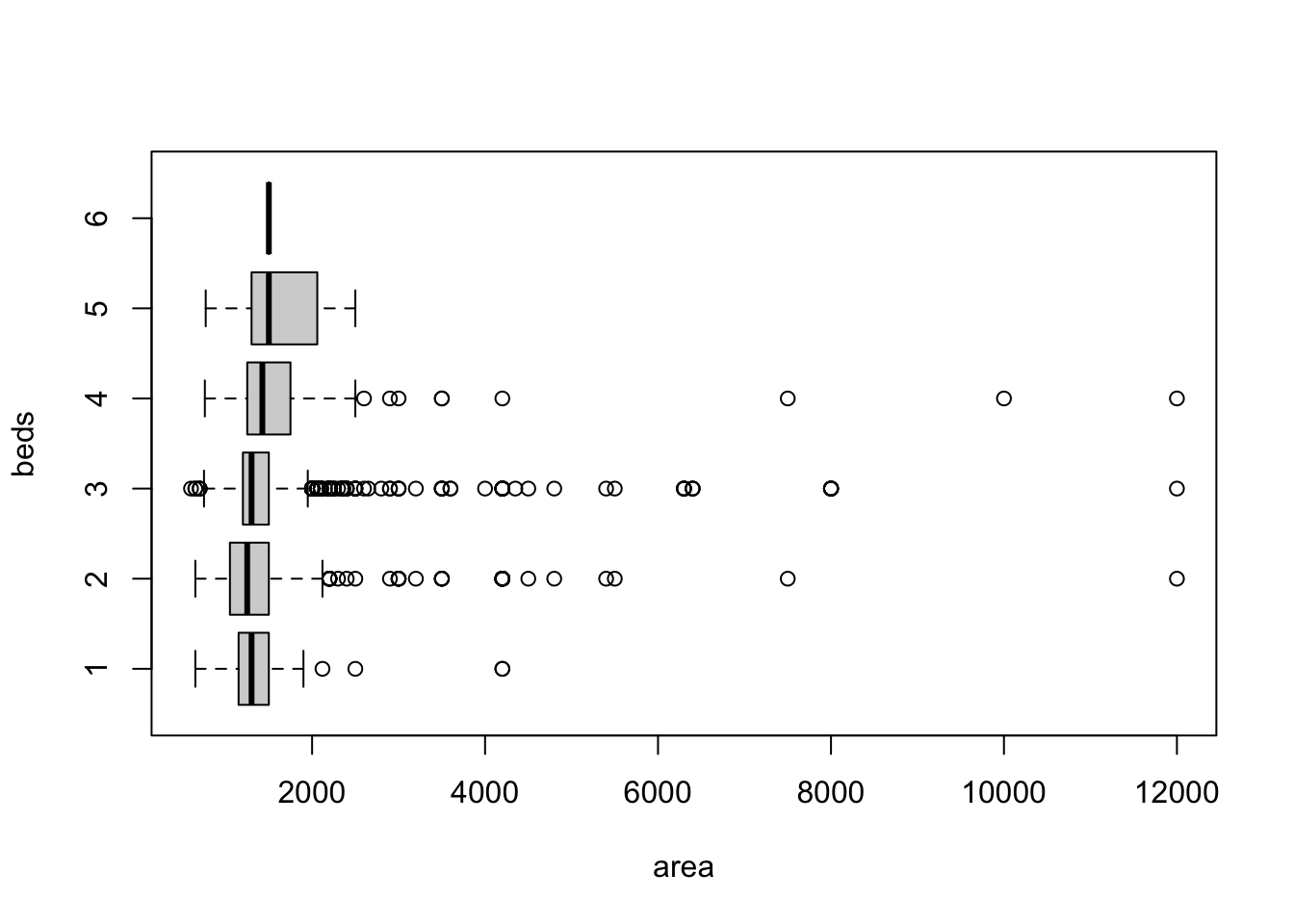
area seems to have a longer positive tail than the negative tail in each subgroup. 12000 sqft is unusually large for a 2/3 bedroom apartment. (To put that into perspective, a basketball court is 4700 sqft). Keeping in mind that these entries are originally created by the property owners from a third world country, it might be the case that some of the values were incorrectly put down. Let’s look at additional attributes of a single row to see whether we can cross-check.
cat(paste(sprintf("%s = %s",
                  names(property_data[1,]),
                  as.character(property_data[1,])),
          collapse = "\n"))
title = To Get A Trouble Free Life You Can Take Rent This 1600 Sq Ft House In Uttara 12
beds = 3
bath = 3
area = 1,500 sqft
address = Priyanka City, Sector 12, Uttara, Dhaka
type = Apartment
purpose = For Rent
floorPlan = https://images-cdn.bproperty.com/thumbnails/1543504-240x180.webp
url = https://www.bproperty.com/en/property/details-5454098.html
lastUpdated = July 29, 2022
price = 30 Thousand
lon = 90.3797847
lat = 23.8685318First thing to notice here is that the area information is embedded in the title. The second thing is that the two information do not match even though the difference is small. Let’s quickly look at how many entries actually have the “sq” or “ft” pattern in them.
(area_embedded_in_title <- property_data_sf$title %>% tolower() %>% grepl(" sq| ft", .) %>% summary()) Mode FALSE TRUE
logical 976 5052 About 83.8088918 % of the rows have the area value embedded in the title. That is even more than the number of rows that have a valid value in the area attribute (4055 ). Let’s try to extract that information.
Let’s look at a few title first that fits the pattern.
(title_vector <- property_data_sf[(property_data_sf$title %>% tolower() %>% grepl(" sq| ft", .)),]$title) %>% head(10) [1] "To Get A Trouble Free Life You Can Take Rent This 1600 Sq Ft House In Uttara 12"
[2] "Visit This 1400 Square Feet Apartment Which Is Vacant For Rent In Maghbazar"
[3] "1500 Sq Ft Apartment Is Up For Rent In Bashundhara, Near Atimkhana Madrasa."
[4] "Check This Beautiful 1250 Sq Ft Flat For Rent At Banasree"
[5] "At Hatirpool 1180 Square Feet Flat For Rent Close To Dhanmondi Ideal College"
[6] "Check This Apartment For Rent Which Is Covering An Area Of 3000 Sq Ft In Baridhara"
[7] "See, this 1807 SQ Ft beautiful apartment and make it your new home which is up for rent in Mohammadpur nearby Baitus Salam Jame Masjid."
[8] "Properly-constructed 1950 SQ FT flat is now offering to you in Bashundhara R-A for rent"
[9] "800 Sq Ft Apartment For Rent In Dakshin Khan"
[10] "Offering You 2200 Sq Ft Amazing Apartment For Rent In Mirpur DOHS" The area size precedes the word containing sq/ft in all the 10 instances above. If we tokenize a title by splitting the string by whitespace and find the index of the token containing sq/ft, then one less than that index is what we are looking for. Let’s define a function that will do this for us.
extract_area <- function(string) {
  tokens <- unlist(strsplit(tolower(string), " "))
  indices <- which(grepl("^sq|^ft", tokens[2:length(tokens)]))
  # return(length(indices))
  index <- indices[1] + 1
  # return(index)
  # return(tokens[index-1])
  area_size <- gsub("[^[:digit:]]", "", tokens[index-1])
  area_size <- gsub(',', '', area_size)
  return(as.numeric(area_size))
}
Before applying it on property_data_sf, let’s verify it’s effectiveness in title_vector. I apply extract_area on title_vector and summarize the result.
#extracted_areas <- purrr::map(title_vector, purrr::possibly(.f = extract_area, otherwise = NA))
extracted_areas <- unlist(lapply(title_vector, extract_area))
summary(extracted_areas)
Min. 1st Qu. Median Mean 3rd Qu. Max. NA's
300 800 1200 1314 1550 6600 1 From the summary, it looks like we have only 1 NA value which means we could not extract area information from that row. Let’s see the title of that row.
title_vector[extracted_areas %>% is.na()][1] "Ready Flat Is Now For Rent In Mohammadpur Nearby Mohammadpur Tokyo Square"“Tokyo Square” is a residential area in Dhaka City and this threw off the extract_area function which was unable to convert “Tokyo” to numeric. This is an acceptable failure.
Now, let’s modify the function extract_area to make it work in cases where there is no sq/ft in the title and after that we will directly apply it on the title attribute of property_data_sf.
extract_area <- function(string) {
  tokens <- unlist(strsplit(tolower(string), " "))
  indices <- which(grepl("^sq|^ft", tokens[2:length(tokens)]))
  if (length(indices)<1) {
    return(NA)
  }
  # return(length(indices))
  index <- indices[1] + 1
  # return(index)
  # return(tokens[index-1])
  area_size <- gsub("[^[:digit:]]", "", tokens[index-1])
  area_size <- gsub(',', '', area_size)
  return(as.numeric(area_size))
}property_data_sf$area_extracted <- unlist(lapply(property_data_sf$title, extract_area))
summary(property_data_sf$area_extracted) Min. 1st Qu. Median Mean 3rd Qu. Max. NA's
300 800 1200 1314 1550 6600 977 Let’s see the correlation of area_extracted with other 3 attributes.
cor(property_data_sf[c('beds', 'bath', 'area_extracted', 'rent')] %>% filter(!is.na(area_extracted)) %>% st_drop_geometry()) beds bath area_extracted rent
beds 1.0000000 0.7858722 0.7425423 0.4588450
bath 0.7858722 1.0000000 0.7694966 0.4665285
area_extracted 0.7425423 0.7694966 1.0000000 0.8172428
rent 0.4588450 0.4665285 0.8172428 1.0000000Awesome! The new area is highly correlated with beds, bath, and rent. Let’s look at the boxplot of area_extracted ~ beds to get an idea of what changed.
boxplot(area_extracted ~ beds, property_data_sf, horizontal=TRUE)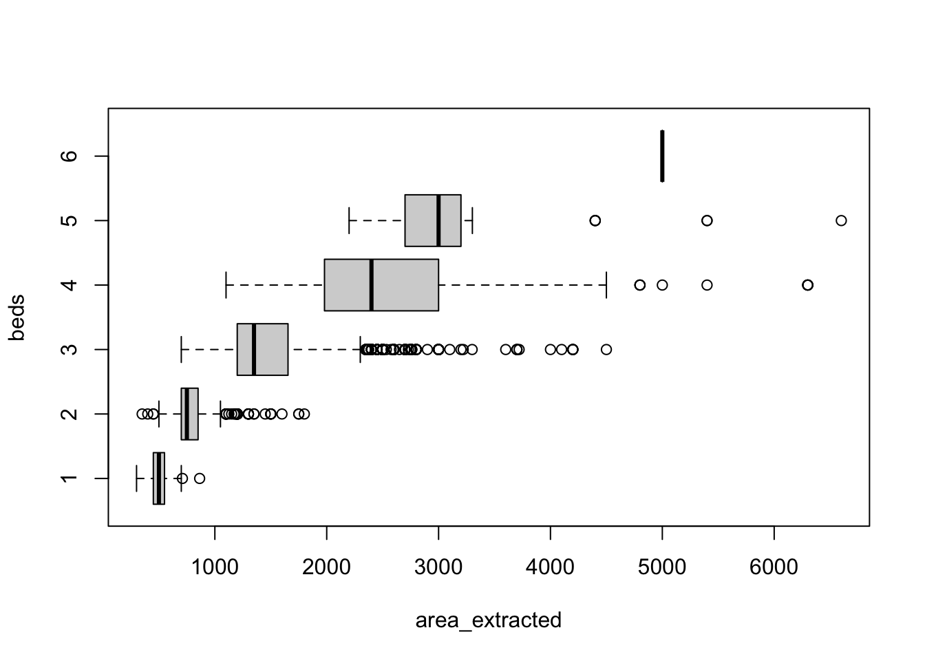
The positive tail in each group has shrunk and the values make realistic sense. The following is my hypothesis on why area_extracted turned out to be more realistic than the original column area. Title is a character string and it represents a summary of the property at a glance. That’s why most property owners were careful in writing it down. The area information was a numeric field that received less attention and as a result generated unreliable values. We will proceed with area_extract so let’s rename the variables.
property_data_sf <- property_data_sf %>% rename(area_from_data = area) %>% rename(area = area_extracted)5051 is enough records for us to work with for now. On a later update, I will try to do geospatial interpolation to find area of the missing values.
The usual approach to apartment rental cost analysis is to compare rent per square feet of the data entries. Let’s mutate a rent_per_sqft column.
property_data_sf$rent_per_sqft <- property_data_sf$rent / property_data_sf$areaWe want to do a comparison among the ADMIN4 areas in term of rent_per_sqft. Let’s group the data by ADM4_PCODE that we added before and calculate mean of the rent_per_sqft for each ADMIN4 area.
mean_rent_per_sqft <- property_data_sf %>%
  st_drop_geometry() %>%
  group_by(ADM4_PCODE) %>%
  summarise(rent_per_sqft = mean(rent_per_sqft, na.rm=TRUE))
summary(mean_rent_per_sqft$rent_per_sqft)
Min. 1st Qu. Median Mean 3rd Qu. Max. NA's
11.54 16.67 20.01 21.19 23.30 51.95 2 There are 2 NA values which means for 2 areas we had no entries with a valid rent_per_sqft value. Let’s drop those 2 areas from mean_rent_per_sqft.
mean_rent_per_sqft <- mean_rent_per_sqft %>% filter(!is.na(rent_per_sqft))[NOTE: I want to add a boxplot/raincloud of rent_per_sqft grouped by ADM3_PCODE later]
We want this information to actually be in the shape_file_4p sf. Let’s copy it there and visualize.
shape_file_4p$rent_per_sqft <- mean_rent_per_sqft$rent_per_sqft[match(shape_file_4p$ADM4_PCODE, mean_rent_per_sqft$ADM4_PCODE)]
plot((shape_file_4p %>% filter(!is.na(rent_per_sqft)))['rent_per_sqft'])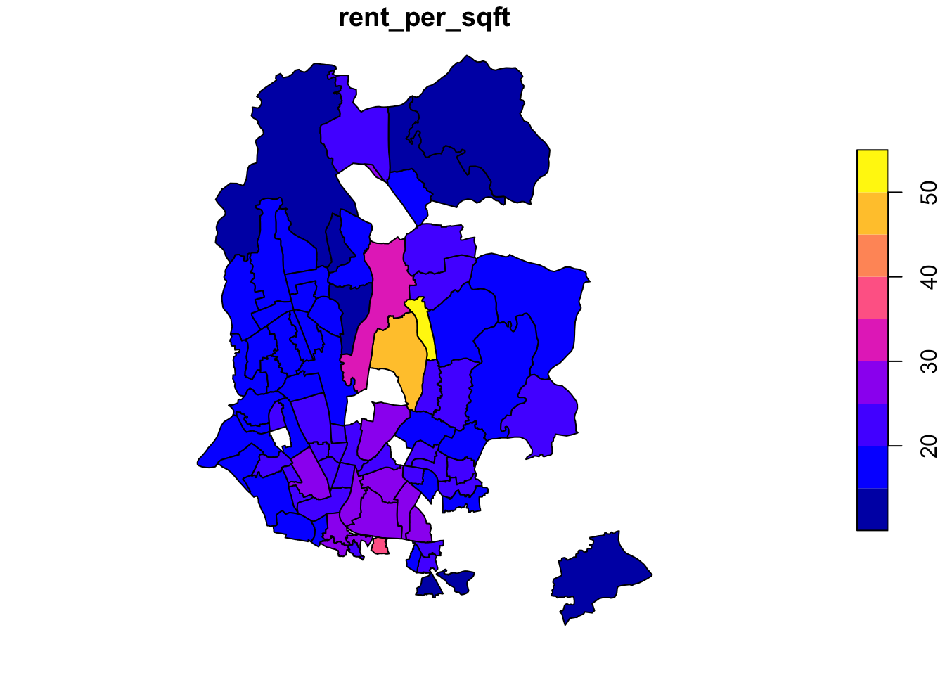
Few things to note here.
The rent_per_sq_ft is homogeneous across most regions except for a few ADMIN4 area in the middle. Those belong to the corporate portion of the city. But it is hard to get a sense of the level of the disparity among the areas from the color value.
I expected some of the areas at the periphery to not have enough information which turned out to be true. Looking at the south portion of the city this effect becomes obvious.
Some middle areas also seem to have no rental property listed. One of them situates the Airport, another is the industrial area.
Now I want to see the rent_per_sqft in a 3D setting to properly assess the disparity.
First, I will load the stars library and rasterize the spatial shape_file_4p.
shape_file_4p <- shape_file_4p %>%
  subset(!is.na(rent_per_sqft))
shape_file_4p$rent_per_sqft <- shape_file_4p$rent_per_sqft * 30library(stars)
grd = st_as_stars(st_bbox(shape_file_4p %>% dplyr::select(rent_per_sqft, geometry)), nx=2500, ny=2500)
raster_map <- st_rasterize(shape_file_4p %>% dplyr::select(rent_per_sqft, geometry), grd)Let’s use the cool rayshader library to plot this raster map.
library(rayshader)

r <- rast(raster_map)
elmat = raster_to_matrix(r)
Also, I want to overlay a streetmap picture of Dhaka over the rayshader11 3D map for the inhabitants to quickly have an idea which portion is actually which area. This is a non-standard step but it ended up looking good so I am keeping it like this. Due to space constraint, I am not adding the steps of actually downloading the picture from ArcGIS but I followed the steps from this brilliant tutorial12.
overlay_file <- "images_dhaka.png"
overlay_img <- png::readPNG(overlay_file)
Let’s finally draw the 3D map.
elmat %>%
  sphere_shade(texture = "imhof2") %>%
  add_overlay(overlay_img, alphalayer = 1.0) %>%
  add_shadow(ray_shade(elmat, zscale = 3), 0.5) %>%
  add_shadow(ambient_shade(elmat), 0) %>%
plot_3d(elmat, zscale = 2, fov = 0, theta = 45, zoom = 0.75, phi = 45, windowsize = c(1600, 1600))render_snapshot('~/Desktop/dhaka_3d.jpg')References
1
Pebesma, Edzer (2018) “Simple Features for R: Standardized Support for Spatial Vector Data.” The R Journal, 10(1), pp. 439–446. [online] Available from: https://doi.org/10.32614/RJ-2018-009
2
Hijmans, Robert J. (2023) Raster: Geographic data analysis and modeling, [online] Available from: https://CRAN.R-project.org/package=raster
3
Wickham, Hadley, François, Romain, Henry, Lionel, Müller, Kirill and Vaughan, Davis (2023) Dplyr: A grammar of data manipulation, [online] Available from: https://CRAN.R-project.org/package=dplyr
4
Bivand, Roger, Nowosad, Jakub and Lovelace, Robin (2022) spData: Datasets for spatial analysis, [online] Available from: https://CRAN.R-project.org/package=spData
5
Hijmans, Robert J. (2023) Terra: Spatial data analysis, [online] Available from: https://CRAN.R-project.org/package=terra
6
Fellows, Ian and JMapViewer library by Jan Peter Stotz, using the (2019) OpenStreetMap: Access to open street map raster images, [online] Available from: https://CRAN.R-project.org/package=OpenStreetMap
7
Mark Padgham, Bob Rudis, Robin Lovelace and Maëlle Salmon (2017) Osmdata, The Open Journal. [online] Available from: https://doi.org/10.21105/joss.00305
8
Cheng, Joe, Karambelkar, Bhaskar and Xie, Yihui (2022) Leaflet: Create interactive web maps with the JavaScript ’leaflet’ library, [online] Available from: https://CRAN.R-project.org/package=leaflet
9
Exchange, Humanitarian Data (n.d.) “Bangladesh - subnational administrative boundaries.” [online] Available from: https://data.humdata.org/dataset/cod-ab-bgd?force_layout=desktop
10
Kaggle (n.d.) “8K+ property listing data in bangladesh.” [online] Available from: https://www.kaggle.com/datasets/ijajdatanerd/property-listing-data-in-bangladesh
11
Morgan-Wall, Tyler (2023) Rayshader: Create maps and visualize data in 2D and 3D,
12
Morgan-Wall, Tyler (2023) “Tutorial: Adding open street map data to rayshader maps in r.”